
Rethinking RF and analog front ends for smarter edge AI


 KEY TAKEAWAYS:
- RF and AFE design are becoming one signal chain
- Each edge AI application demands RF and analog design variations
- A co-design checklist helps engineers develop faster
Industrial IoT is evolving fast. Sensors are no longer just feeding PLCs and SCADA systems; they are also powering edge AI that needs richer, more nuanced data to spot anomalies, drift and emerging failure modes before they become downtime. That raises the bar for how the RF and analog front-end is architected. It needs to be AI-ready from day one rather than retrofitted later.
From industrial IoT signal chain to edge AI pipeline
A typical industrial sensing node includes three layers:
- An RF and analog front-end that interfaces to the physical world and conditions the signal
- A converter and timing chain that digitizes and transports data
- An edge processor that runs AI models and supporting firmware
The RF and AFE front-ends to edge AI-enabled industrial sensing applications
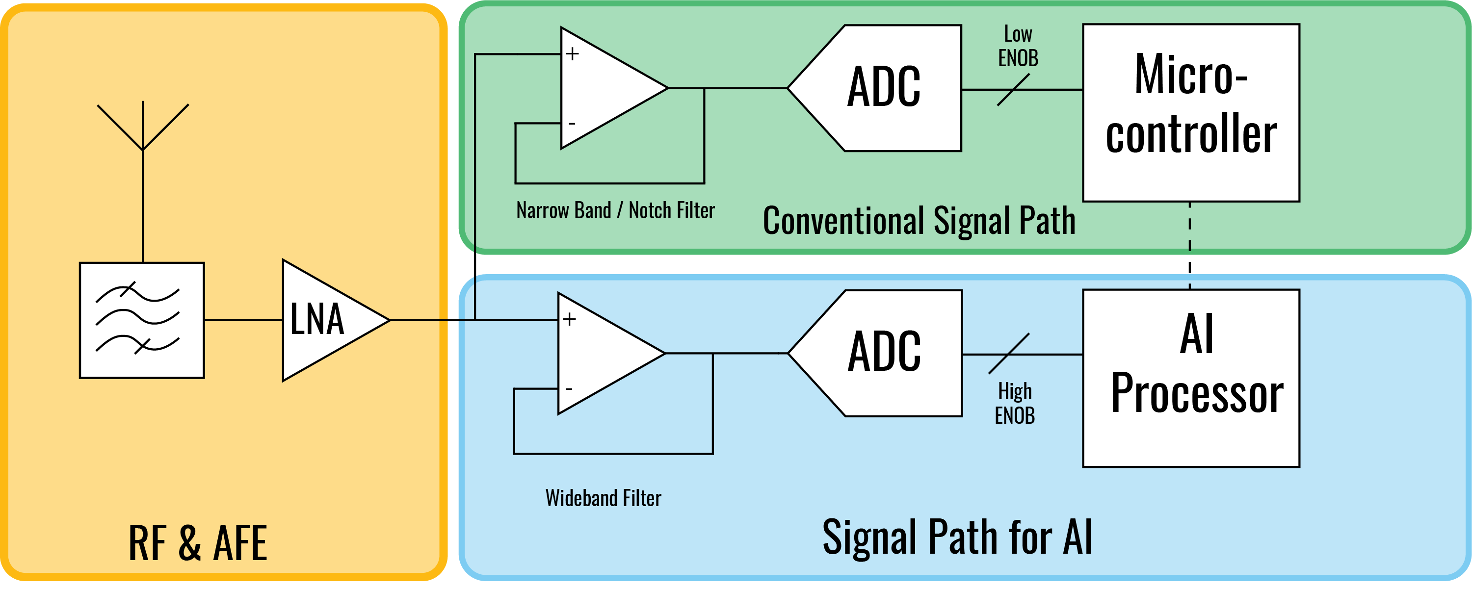
The basic building blocks of a sensor front-end might now drive two signal chains for both conventional and AI-enabled feature detection. (Source: Avnet)
In a traditional design, the front-end delivers “suitable” samples into a control loop. With AI in the path, “suitable” changes. The system must preserve weak harmonics, modulation sidebands, noise characteristics, and phase relationships that AI models may use during both training and inference.
That requirement shows up directly in the noise and resolution budget.
- Threshold-style systems may work with about 40–50 dB SNR.
- AI-oriented feature extraction often benefits from roughly 60–80 dB effective SNR so that weak components remain visible above the noise floor.
Using the standard quantization-noise-limited signal/noise ratio (SNR) for an ideal N-bit ADC with a full-scale sine input:
SNR ≈ 6.02N + 1.76 dB
This translates to roughly 10 to 13 effective number of bits measured at the frequencies of interest, not the nominal resolution at DC.
Thinking in terms of an intelligence pipeline leads to different choices. Bandwidth and dynamic range are sized not only for today’s thresholds but also for the features future models may uncover. “AI-ready” does not mean maximum bandwidth; it means preserving the right information with sufficient fidelity.
Use case 1: Vibration monitoring
Wireless vibration sensing on rotating machinery is a textbook RF and AI co-design problem. Early-stage bearing and gear faults can sit 20-40 dB below dominant vibration components, yet those weak signatures are often the signals that matter most for predictive maintenance.
Consider a simple numeric example:
- Peak vibration under full load is mapped to 0 decibels relative to full-scale (dBFS)
- Early fault signatures appear around −40 dBFS
- To maintain about 20 dB margin, the in-band noise floor should be below −60 dBFS
That implies at least about 10 effective number of bits (ENOB) in-band, and more realistically 11-12 bits once analog noise and distortion are included in the full error budget.
Assume a pump needs 0-500 Hz vibration data for control. A traditional design might choose about 500 Hz signal bandwidth and a sampling rate modestly above Nyquist, such as around 1.2 kS/s. Once AI enters the picture, broader bandwidth often becomes useful.
- AI-oriented bandwidth: 3-5 kHz to capture bearing harmonics, resonance bands, and sidebands
- Sampling rate: 10-20 kS/s
The data rate rises by roughly an order of magnitude. In return, the system can support envelope detection of higher-frequency resonance bands, sideband analysis around shaft and bearing defect frequencies, and richer feature sets for machine learning models. Power consumption tends to rise with sample rate for a given ADC architecture, so designers often combine higher-rate bursts with duty cycling or local feature extraction to stay within energy targets.
Dynamic range can quickly become the limiting factor. Real machines can move from roughly −50 dBFS at idle to 0 dBFS under load. A fixed-gain front-end forces a tradeoff between fault visibility and overload margin.
Common responses include dual-range programmable gain amplifiers (PGAs), for example ×1 and ×8, which extend usable span by about 18 dB, along with gain-state tagging so downstream models can normalize correctly.
Slow automatic gain control (AGC) loops with time constants much longer than fault transients also help the system’s detection of impulses. Feature-based compression at the node can reduce a 16-bit, 10 kS/s stream at about 160 kbps down to roughly 100–500 bps when using spectral features, band energies, and statistical descriptors.
Use case 2: Condition monitoring
RF-based condition monitoring treats the channel as a sensor. Small perturbations in amplitude, phase, and frequency can carry information about the environment, load, or structural changes, provided the signal chain can resolve them.
The variations of interest are often small:
- Amplitude changes: less than 1 dB
- Phase shifts: a few degrees or less
- Frequency offsets: tens to hundreds of hertz on MHz carriers
To resolve these reliably, approaches based on received signal strength indicators (RSSI) typically need better than 0.5 dB repeatability, while phase-based systems require local oscillator (LO) phase noise and stability better than the effect being measured. As a simple benchmark, at 2.4 GHz a 1° phase shift corresponds to about 1.16 ps of timing variation. Maintaining that level of effective stability over temperature and aging calls for careful LO design and, in many cases, periodic calibration.
If the system captures baseband I and Q, a 12-bit ADC has an ideal SNR of about 74 dB for a full-scale sine input, often rounded to about 70 dB in first-pass system estimates. Practical ENOB values of 9–11 bits reduce that to roughly 56–68 dB once noise and distortion are included. This provides a useful lower bound set by quantization and front-end non-idealities on the smallest channel variation the baseband chain can expose.
Rather than exposing only decoded packets or aggregate metrics, RF and AI systems can surface richer structures such as decimated I/Q snapshots, for example 1–10 ms windows, or channel impulse response vectors. A ten-fold reduction in sample rate using decimation can preserve much of the relevant structure while keeping data volumes manageable, provided the retained bandwidth still covers the features of interest.
Use case 3: Low-power asset sensing
Sub-GHz frequency shift keying (FSK) and LoRaWAN-based asset sensors operate under tight constraints. Data rates are often in the range 0.3–50 kbps, duty-cycle limits in several commonly used EU868 sub-bands are 1 percent, and battery life targets often span 5–10 years. Design teams must squeeze maximum insight out of every microamp and every transmitted bit.
A representative node budget might look like this:
- MCU plus ADC active current: 5–15 mA
- Sleep current: below 10 µA
- Radio transmit current: 30–120 mA in short bursts
On the RF side, a LoRaWAN uplink payload might be around 50 bytes, or roughly 400 bits. Raw vibration sampled at 12-bit, 5 kS/s is about 60 kbps, so the required compression ratio can easily exceed 100:1.
Strategies to bridge that gap include local feature extraction, event-triggered reporting, and sparse high-rate windows such as 1 second of sampling every 10 minutes. Sampling for 1 second every 600 seconds yields a sampling duty cycle of about 0.17 percent, which makes higher instantaneous sampling rates and bandwidth feasible while keeping long-term energy use and regulatory limits under control.
RF and AI sensing co-design checklist
| Design focus | ractical guideline |
|---|---|
| Physics and features | Map target effects to bandwidth and SNR; for −40 dB sidebands, aim for at least about 60 dB effective SNR. |
| Bandwidth planning | Treat Nyquist as a floor, not a target; consider 5–10X oversampling when power allows. |
| Dynamic range and ENOB | Use in-band ENOB derived from measured SINAD, not headline DC resolution or nominal converter bits. |
| Gain control metadata | Log gain-state changes so AI models do not confuse them with real faults. |
| Edge processing level | Target 10X to 1000X compression using features and event-driven reporting. |
| Timing and alignment | Use sub-sample synchronization for phase-sensitive and RF-based sensing. |
| Environmental effects | Budget for some ENOB loss over temperature and aging, and include calibration hooks where drift matters. |
| Field data iteration | Use deployment data to refine SNR targets, bandwidth, and feature selection |
When the RF and analog front-end is treated as a core part of the AI system, not just a data source, industrial sensing nodes move beyond simple threshold monitoring. They become instruments for early detection, predictive maintenance, and deeper operational insight, grounded in measurable signal integrity.

